Overview
This guide explains how to analyze time-series fluorescence data from plate reader expression experiments using the open-source Nucleus Cell Development Kit (CDK). Here, we’ll cover how to load, normalize, visualize, and fit your data (see DevNote), as well as describe the resulting summary statistics.
The CDK is available on PyPi for install on your own computer (requires Python 3.11+ and the poetry package).
It is the cytosol counterpart to Analyzing Microscopy Data. Reference material is in the cytosol API reference.
1. Setup
First, import the necessary libraries. The platereader module from the CDK contains specialized functions for loading plate reader data, performing kinetic analysis, and visualization. By convention, we import platereader as pr.
%load_ext autoreload
%autoreload 2

import pandas as pd
import seaborn as sns
import matplotlib.pyplot as plt

# Import the cdk platereader module
from cdk.instruments import platereader as pr
2. Load Data
Load your plate reader output and merge it with the platemap (see DevNote) that describes your experimental conditions.
data_file: path to the output file from a plate reader experiment. Currently only BioTek plate readers are supported.platemap_file: path to a platemap CSV mapping eachWellto its experimental conditions. See the platemap tutorial for the expected format.
Call load_platereader_data() to parse the file:
# Specify file paths
data_file = "path/to/data.txt"
platemap_file = "path/to/platemap.csv"

# Load data
result = pr.load_platereader_data(
    data_file=data_file,
    platemap_file=platemap_file,
    platereader="biotek"
)
The output is a PlateReaderResult object: a list-like collection of PlateReaderData blocks. If you did more than one read on the plate (multiple gains, or different ex/em spectra), each read is a separate block. Print result to see what’s inside:
print(result)PlateReaderResult with the following 2 blocks:
0: (1533, 54) kinetic read with reads: GFP-G70:485,528 (Fluorescence) (Plate 'Plate 1')
1: (1533, 54) kinetic read with reads: GFP-Gext:485,528 (Fluorescence) (Plate 'Plate 1')The output lists all of the blocks in the data file. For each block, you can see its index, the type of experiment stored (here, kinetic), the dimensions of the underlying DataFrame, the reads recorded and their measurement modalities, and the ID of the plate used.
Here, there are two reads of a single plate with different gains and the same excitation/emission spectra. To work with a single read, choose its index (e.g., the GFP-Gext read is block index 1):
desired_index = 1
data = result[desired_index]
You can see the underlying data with data.view() (which returns a Pandas DataFrame):
# Show the first five rows:
data.view().info()
<class 'pandas.core.frame.DataFrame'>
RangeIndex: 1533 entries, 0 to 1532
Data columns (total 42 columns):
# Column Non-Null Count Dtype
--- ------ -------------- -----
0 Date 1533 non-null datetime64[ns]
1 Experiment 1533 non-null object
2 Well 1533 non-null object
3 Name 1533 non-null object
4 Type 1533 non-null object
5 Time 1533 non-null timedelta64[ns]
6 Data 1533 non-null int64
7 Data_normalized 1533 non-null float64
8 Read 1533 non-null object
9 Read Name 1533 non-null object
10 Reader Type 1533 non-null object
11 Reader ID 1533 non-null object
12 Plate Type 1533 non-null object
13 Plate ID 1533 non-null object
14 Start Time 1533 non-null datetime64[ns]
15 Read Modality 1533 non-null object
16 Gain 1533 non-null object
17 Excitation Wavelength (nm) 1533 non-null int64
18 Excitation Bandwidth (nm) 1533 non-null object
19 Excitation Optics 1533 non-null object
20 Emission Wavelength (nm) 1533 non-null int64
21 Emission Bandwidth (nm) 1533 non-null int64
22 Emission Optics 1533 non-null object
23 Read Geometry 1533 non-null object
24 Read Height (mm) 1533 non-null object
25 PMix ID 1314 non-null object
26 [PMix] (mg/mL) 0 non-null float64
27 Ribosome ID 0 non-null float64
28 [Ribosome] (uM) 0 non-null float64
29 SMS ID 1314 non-null object
30 tRNA ID 1095 non-null object
31 [tRNA] (ug/uL) 1095 non-null float64
32 DNA ID 1314 non-null object
33 [DNA] (ng/uL) 1314 non-null float64
34 PMix Vol (uL) 1314 non-null float64
35 Ribosome Vol (uL) 0 non-null float64
36 SMS Vol (uL) 1314 non-null float64
37 tRNA Vol (uL) 1314 non-null float64
38 DNA Vol (uL) 1314 non-null float64
39 RNase Inhib Vol (uL) 1314 non-null float64
40 Water vol (uL) 1314 non-null float64
41 Rxn Volume (uL) 1314 non-null float64
dtypes: datetime64[ns](2), float64(14), int64(4), object(21), timedelta64[ns](1)
memory usage: 503.1+ KBThe dataset contains information from the platemap and metadata extracted from the plate reader’s output, in long format. Each row represents a single measurement, where:
Timerepresents the time point of the measurement relative to the start of the experiment,Readis the label of the read applied by the plate reader configuration, andDatais the raw value of the measurement.
3. Plot Raw Curves
First, visualize your data. You can do this by calling data.plot(). By default, one curve is plotted for each distinct Name in the platemap. The band shows a bootstrapped 95% confidence interval of the mean across wells with that Name.
Passing style='Type' assigns different line styles for the different sample types that appear in your platemap (Sample, Standard, Blank, etc. as defined in the platemap standard). Line styles by type makes it easy to spot controls, catch outliers, failed reactions, or unexpected behavior before fitting data.
data.plot(style='Type')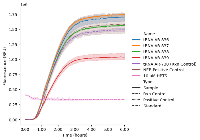
We can see that our Samples show typical behavior and that the standard (here, HPTS) is stable, thus we can safely normalize our data.
4. Normalize Data
Instead of performing your analyses on the raw units output by the plate reader, we recommend first normalizing to a standard so values are comparable across experiments and instruments.
The function data.normalize('<standard name>') takes the time average of each well labeled as a Standard at the end of the run (1 hour by default), then divides all data by that mean.
The name you pass as an argument to data.normalize() must match the standard’s Name column from your platemap. You can check the name of your standards this way:
platemap = data.platemap
standards = platemap[platemap['Type']=='Standard']
standards['Name'].unique()
array(['10 uM HPTS'], dtype=object)Then, call data.normalize():
data = data.normalize('10 uM HPTS')NOTE: you need to save the output of this transformation — it does not happen in-place!
Now replot to see your normalized data. We exclude the standard from the plot using exclude_types=['Standard']:
g = data.plot(style='Type', exclude_types=['Standard'])
# To save the output:
# g.savefig('after-normalization.png',dpi=300)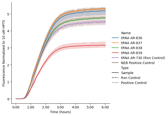
The plot y-axis label will automatically update to indicate that your data have been normalized and will indicate the name of the standard used.
5. Kinetic Analysis
Now we’re ready to do our kinetic analysis.
data.fit_kinetics() fits a sigmoid-with-drift curve to each well (grouped by unique well identifiers: Experiment, Well, Read, and Reader ID by default) and extracts interpretable kinetic parameters.
The model is:
with parameters:
: steady-state level (asymptote)
: growth rate (steepness)
: inflection point (time of maximum velocity)
: drift rate (linear signal change after steady-state)
: drift onset time
See the DevNote on kinetic analysis for more details.
Metrics extracted:
Max Velocity: maximum rate of fluorescence increase (slope at inflection point)
Lag Time: time to reach the exponential phase
Steady State: final fluorescence level
Completion Time: time to reach 95% of the asymptote
Drift: rate of signal decay or increase after steady-state
R²: goodness of fit; “Good Fit” is
Trueif
Run the kinetic analysis:
kinetics = data.fit_kinetics()fit_kinetics() returns a Kinetics object. Its .summary property is a tidy table of the fitted parameters and quality metrics per group (all-null columns dropped):
kinetics.summary| Well | Name | Max Velocity | Max Velocity Time | Lag Time | Steady State | Completion Time | Completion Threshold | Drift | Fit Function | R^2 | Good Fit | Normalized to | |
|---|---|---|---|---|---|---|---|---|---|---|---|---|---|
| 0 | B2 | tRNA AR-836 | 2.49 | 0 days 01:33:15 | 0 days 00:33:09 | 4.74 | 0 days 03:01:44 | 0.95 | 0.07 | sigmoid_drift | 1.00 | True | 10 uM HPTS |
| 1 | B4 | tRNA AR-837 | 2.67 | 0 days 01:33:35 | 0 days 00:34:38 | 4.99 | 0 days 03:00:24 | 0.95 | 0.07 | sigmoid_drift | 1.00 | True | 10 uM HPTS |
| 2 | B6 | tRNA AR-838 | 2.44 | 0 days 01:32:35 | 0 days 00:34:21 | 4.50 | 0 days 02:58:17 | 0.95 | 0.06 | sigmoid_drift | 1.00 | True | 10 uM HPTS |
| 3 | B8 | tRNA AR-839 | 1.68 | 0 days 01:32:00 | 0 days 00:37:35 | 2.89 | 0 days 02:52:07 | 0.95 | 0.03 | sigmoid_drift | 1.00 | True | 10 uM HPTS |
| 4 | B10 | tRNA AR-730 (Rxn Control) | 2.37 | 0 days 01:30:01 | 0 days 00:33:50 | 4.22 | 0 days 02:52:45 | 0.95 | 0.07 | sigmoid_drift | 1.00 | True | 10 uM HPTS |
| 5 | B12 | NEB Positive Control | 2.66 | 0 days 01:35:50 | 0 days 00:45:09 | 4.27 | 0 days 02:50:26 | 0.95 | 0.09 | sigmoid_drift | 1.00 | True | 10 uM HPTS |
| 6 | D2 | tRNA AR-836 | 2.64 | 0 days 01:31:44 | 0 days 00:32:12 | 4.97 | 0 days 02:59:23 | 0.95 | 0.08 | sigmoid_drift | 1.00 | True | 10 uM HPTS |
| 7 | D4 | tRNA AR-837 | 2.79 | 0 days 01:32:13 | 0 days 00:34:27 | 5.10 | 0 days 02:57:16 | 0.95 | 0.07 | sigmoid_drift | 1.00 | True | 10 uM HPTS |
| 8 | D6 | tRNA AR-838 | 2.52 | 0 days 01:32:00 | 0 days 00:34:31 | 4.58 | 0 days 02:56:37 | 0.95 | 0.06 | sigmoid_drift | 1.00 | True | 10 uM HPTS |
| 9 | D8 | tRNA AR-839 | 1.84 | 0 days 01:30:32 | 0 days 00:35:41 | 3.20 | 0 days 02:51:17 | 0.95 | 0.04 | sigmoid_drift | 1.00 | True | 10 uM HPTS |
| 10 | D10 | tRNA AR-730 (Rxn Control) | 2.41 | 0 days 01:28:51 | 0 days 00:32:20 | 4.31 | 0 days 02:52:03 | 0.95 | 0.07 | sigmoid_drift | 1.00 | True | 10 uM HPTS |
| 11 | D12 | NEB Positive Control | 3.13 | 0 days 01:34:33 | 0 days 00:44:14 | 4.99 | 0 days 02:48:38 | 0.95 | 0.09 | sigmoid_drift | 1.00 | True | 10 uM HPTS |
| 12 | F2 | tRNA AR-836 | 2.79 | 0 days 01:30:12 | 0 days 00:32:10 | 5.12 | 0 days 02:55:38 | 0.95 | 0.08 | sigmoid_drift | 1.00 | True | 10 uM HPTS |
| 13 | F4 | tRNA AR-837 | 2.77 | 0 days 01:31:33 | 0 days 00:33:22 | 5.10 | 0 days 02:57:12 | 0.95 | 0.07 | sigmoid_drift | 1.00 | True | 10 uM HPTS |
| 14 | F6 | tRNA AR-838 | 2.49 | 0 days 01:30:49 | 0 days 00:33:35 | 4.51 | 0 days 02:55:05 | 0.95 | 0.06 | sigmoid_drift | 1.00 | True | 10 uM HPTS |
| 15 | F8 | tRNA AR-839 | 1.79 | 0 days 01:28:45 | 0 days 00:36:41 | 2.95 | 0 days 02:45:25 | 0.95 | 0.03 | sigmoid_drift | 1.00 | True | 10 uM HPTS |
| 16 | F10 | tRNA AR-730 (Rxn Control) | 2.46 | 0 days 01:28:12 | 0 days 00:32:05 | 4.37 | 0 days 02:50:49 | 0.95 | 0.07 | sigmoid_drift | 1.00 | True | 10 uM HPTS |
| 17 | F12 | NEB Positive Control | 2.52 | 0 days 01:33:54 | 0 days 00:44:03 | 3.98 | 0 days 02:47:18 | 0.95 | 0.08 | sigmoid_drift | 1.00 | True | 10 uM HPTS |
Visualizing fits
The function kinetics.plot() overlays each fitted curve on its raw data so you can confirm the fits are reasonable (high R², smooth curves).
By default, kinetics.plot() facets by Name, where traces of replicate wells of each condition are shown in a single panel with an average fit overlaid:
g = kinetics.plot()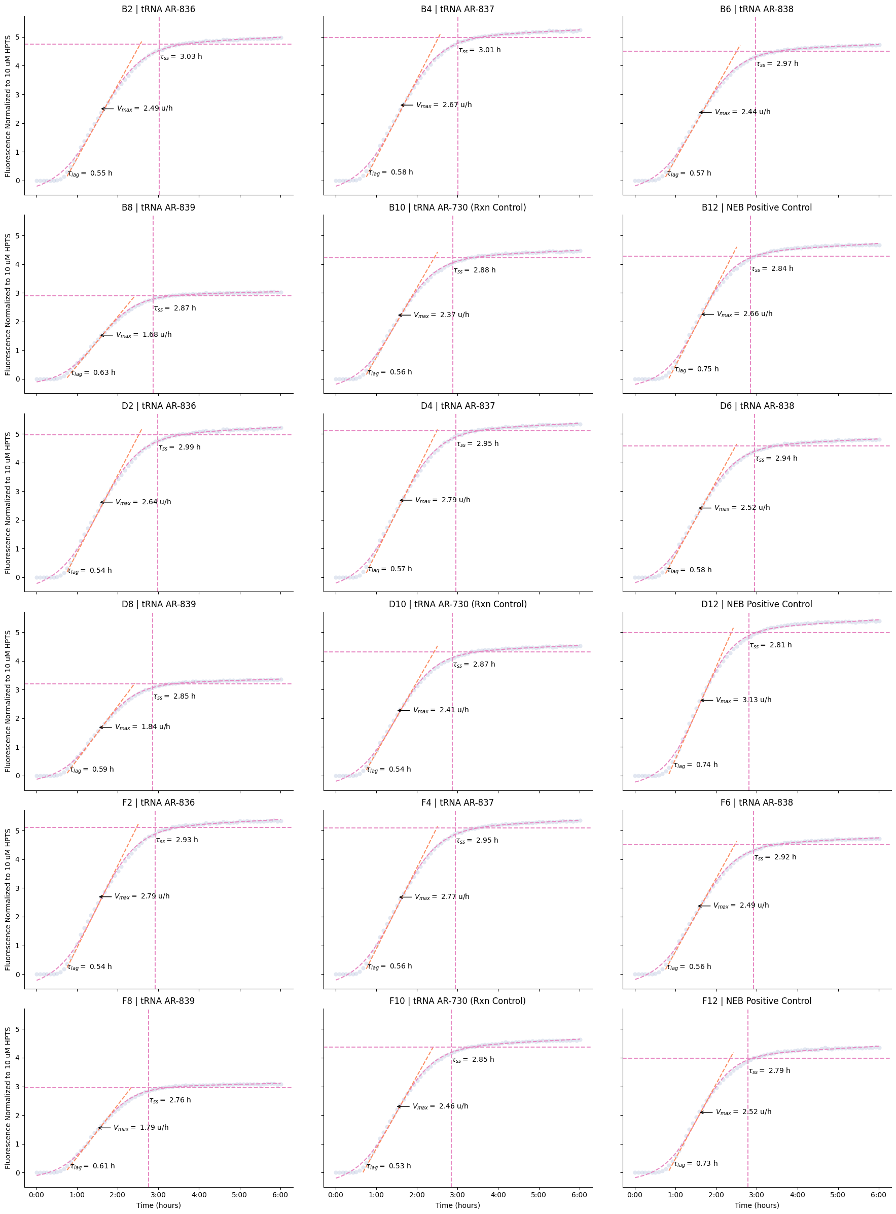
To show the fits to individual replicates separately, facet on Well:
g = kinetics.plot(col="Well")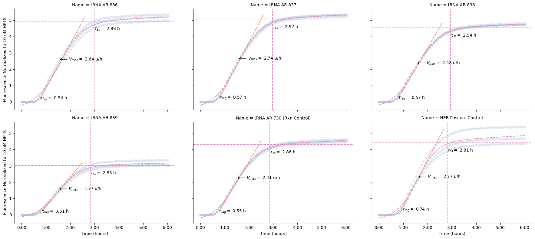
6. Summary Plots
kinetics.plot_summary() produces a multi-panel figure comparing kinetic parameters across conditions: per-experiment time series, in addition to bar plots of steady-state, max velocity, and drift with error bars across technical replicates.
g = kinetics.plot_summary()
# To save:
# g.savefig("data_summary.png", dpi=300)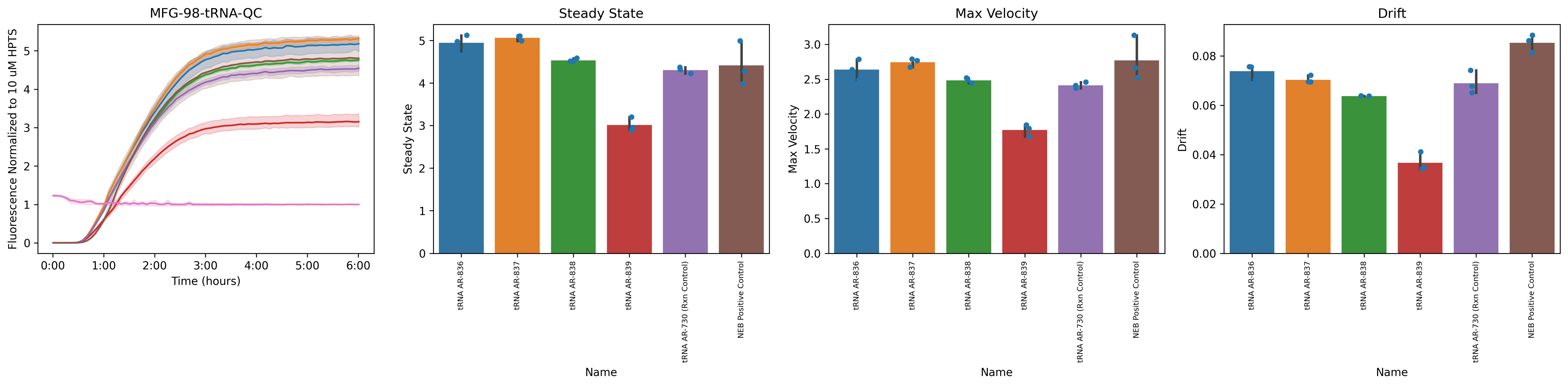
Tips and Troubleshooting
Overflow errors: Wells with
OVRFLWorNaNvalues are automatically excluded from fittingPoor fits (low R²): Inspect raw curves for anomalies (bubbles, evaporation, pipetting errors)
Drift: Sometimes seen in kinetics curves; the default
sigmoid_driftmodel accounts for itMultiple replicates: Always include technical replicates and report error bars
Comparing conditions: Normalize or blank data consistently across all samples